Broad strokes: explaining finite-time blowup by analogy with the Burgers equation.
OpenAI has claimed that their internal model has resolved the question of global existence of smooth solutions to the incompressible (forced) Navier-Stokes equations. The proof is Lean-verified, which is strong evidence for correctness, but as far as I can tell is officially still under review.
In this article, I hope to give the lay reader familiar with basic calculus an intuitive feel for what ‘finite time blow-up’ means for an analyst of partial differential equations (PDEs). I will assume that the reader has basic knowledge of calculus, but no more. Certain facts may be assumed as black boxes for the lay reader.
Before stepping to partial differential equations (PDEs), however, let us stop to smell the ordinary ones (ODEs), in order to pump our intuition. The term ‘ordinary’ refers to the fact that the functions involved are typically derivatives of functions with respect to a single variable, which we can often think of as time, as opposed to PDEs which involve the derivatives of functions of multiple variables. To see the effect of nonlinearity starkly, we compare and contrast the following ODEs:
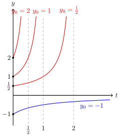
\[y^{\prime}(t)=1,\qquad y^{\prime}(t)=y(t),\qquad y^{\prime}(t)=y(t)^2;\qquad y(0)\in\mathbb R.\]Such a problem is known as an “initial value problem” – the dynamics and starting point are given, and the goal is to determine the trajectory that is forced upon us. The solutions, whenever they exist, are unique (black box: the Picard-Lindelöf/Cauchy-Lipschitz theorem). The first equation is nearly trivial to solve; the solution, as any reader can easily check, is \(y(t)=y(0)+t\). The second equation is linear, i.e. any two solutions can be added or scaled and the result is another solution of the ODE. Since the exponential function is the unique fixed point of the derivative operator up to scaling by a constant factor (exercise left to the reader), solutions are of the form \(y(t)=y(0)\,e^{t}\). In both cases, solutions are mild-mannered and well-defined for all time, given any starting point \(y(0)\in\mathbb R\).
In contrast, the third equation, also known as the Riccati equation, is potentially pathological. The explicit solution is given by
\[y(t)=\frac{y(0)}{1-t\,y(0)},\]which readers can check for themselves. For any given initial value \(y(0)\), this solution is well defined for small enough times, and if \(y(0)\) is negative, then the solution is defined for all positive times. However, if \(y(0)>0\), then the feedback loop pushes \(y\) faster and faster as the denominator approaches zero, and by \(t=y(0)^{-1}\), the solution has shot off to positive infinity, or ‘blown up’. In this case, the solution cannot be defined beyond a certain time \(T^*\). The blow-up criterion is also sharp – if the solution has a finite value at some \(T>0\), then it can be continued for some small interval of time beyond \(T\). Thus, we have a dichotomy: either the solution exists for all time, or approaches infinity in finite time. There is no other possibility.
Evolution equations are typically solved as these sorts of ‘initial value problems’, also known as ‘Cauchy problems’. The Navier-Stokes equations are framed in a similar way. In a precise sense, these PDEs can be conceived of as ODEs in an infinite-dimensional space. This notion of ‘going to infinity’ requires the selection of an appropriate norm, which differs from equation to equation.
The incompressible Navier-Stokes equations,
\[\partial_tu+(u\cdot\nabla)u+\nabla p=f+\nu\Delta u\] \[\nabla\cdot u=0\]describe the evolution of a fluid’s velocity field in space and time as it is pushed around by internal pressure \(p\) and external forces \(f\), as well as accounting for friction, represented by the viscous term \(\nu\,\Delta u\). The ‘incompressible’ term refers to the manner in which the conservation of mass is enforced: fluid packets cannot be squished or stretched in one direction without being stretched or squished respectively in other directions to compensate, and thus exactly maintain their volume through time. This is represented in the ‘divergence free’ constraint \(\nabla\cdot u=0\) on the fluid velocity \(u\).
The full Navier-Stokes equations may be difficult to wrap your head around, so let’s try a simpler model first. Instead of working with fluids, we will work with schmuids. First, in a classic physicist gag, we will ignore friction. Next, we assume there are no external forces, so \(f=0\), and ignore the pressure term, so that \(p=0\) as well. Now, in the original formulation, \(p\) was not independent of \(u\) but implicitly defined in terms of it because of the divergence free condition. So we have to drop the divergence constraint as well. Finally, we assume the simplest possible transcendental aesthetic: just one dimension of space and one of time. Our equation, for \(u:\mathbb{R}\times\mathbb{R}_+\to\mathbb{R}\), now describes the scalar velocity field of the schmuid in space and time:
\[\partial_tu+u\,\partial_xu=0.\]This is also known as the inviscid Burgers equation (please note that it is either “Burgers equation” or “Burgers’ equation”, and not “Burger’s equation”). It is classified as a ‘quasilinear hyperbolic equation’, but we don’t need to worry about the terminology. Typically, the second term is written as \(\partial_x(u^2/2)\), so the equation states that the space-time divergence of the ‘vector field’ \((u,u^2/2)\) is zero.
At first glance, however, it may not be very obvious how to solve even this. Since the non-linearity has been bothering us for so long, we finally get rid of it. Let \(a\in\mathbb{R}\) be a constant, and consider instead the equation
\[\partial_tu+a\,\partial_xu=0,\]also known as a ‘transport equation’; this humble equation contains the seeds of all hyperbolic PDEs, and their characteristic property, the finite speed of propagation.
Mathematically, the transport equation is quite easily solvable if you recall the chain rule for derivatives. Given an initial value \(u_0\) for the Cauchy problem, the scalar field \(u(x,t)=u_0(x-at)\) solves the transport equation with given initial condition, because \(\partial_tu(x,t)=-a\,u_0^\prime(x-at)\) by the chain rule. The solution can be visualised as a profile traveling with speed \(a\), completely unchanged. It is also constant along lines \(x_0+at\); these lines of constancy are known as ‘characteristics’, and can be represented in a space-time diagram as follows, where we take \(a=1\):
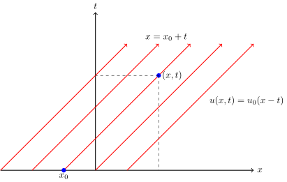
Notice what linearity gets us: since the initial value \(u_0\) is merely translated at a constant speed, the regularity of the solution \(u\) is precisely whatever regularity \(u_0\) has. For later use, note that this form of the solution is true even when \(u_0\) has discontinuities; the ‘solution’ of the Cauchy problem for the transport equation is given by \(u(x,t)=u_0(x-at)\) even when \(u_0\) is discontinuous, since formally defining \(u\) does not assume differentiability or even continuity on the part of \(u_0\).
Suppose a signal travels at speed \(a\) in our one-dimensional spacetime. If the signal packet in space at the initial time is represented by \(u_0(x)\), then at time \(t\), the profile must look like \(u_0(x-at)\) provided the packet itself is invariant under transmission. Thus, signal transmission is precisely described by the linear transport equation. This notion of transport also works if the transport field \(a\) depends on space and time, in which case the characteristics are no longer straight rays, but rather integral curves of \(a\), i.e. solving \(X^\prime(t)=a(X(t),t)\). If instead the characteristic field is given by \(a=u\), as in the case of the Burgers equation, we have that along the characteristic \(X(t)=x_0+u_0(x_0)t\), since \(X^\prime(t)=u(X(t),t)\), the solution is constant:
\[\frac{d}{d\,t}(u(X(t),t))=\partial_tu+X^\prime(t)\partial_xu=\partial_tu+u\,\partial_xu=0.\]Now that we have comprehended the simple transport equation, we can pop back up one level and consider the inviscid Burgers equation instead. If \(u_0\) is identically equal to some constant \(a\), then again all the characteristics are as for the transport equation, and the stationary solution \(u\equiv a\) is the solution to the associated Cauchy problem. The characteristics’ picture still aids us, but now the slope of the characteristics depends on the initial value \(u_0\) at the base point. Thus, \(u\) satisfies a maximum principle: its value at future times never exceeds its maximum value at the initial time.
Consider Lipschitz initial data \(u_0\). If \(u_0\) is a monotone non-decreasing function, i.e. \(u_0(x)\leq u_0(x+h)\) for all \(x\in\mathbb R,h>0\), then two rays emanating from different points in space at the initial time will never meet. This is because the ray from \(x+h\) moves at least as fast as, if not faster than, the ray from \(x\). Furthermore, the set of all rays covers the entirety of the space-time half-plane.
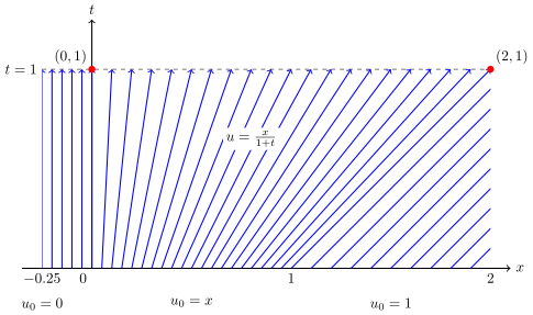
Else, there must be some \(x\in\mathbb R\) and \(h>0\) such that \(u_0(x)>u_0(x+h)\). Hence, the characteristics emanating from \(x,x+h\) respectively clash in finite time, say \(T^*\), yielding the absurd implication that the function is multivalued at and beyond this intersection point, since the characteristics cross each other. As a consequence, the spatial derivative of the solution approaches negative infinity as \(t\uparrow T^*\) (see the figure below), although \(u\) itself stays bounded, by the maximum principle. This is precisely what we mean by ‘blow-up’. The classical notion of a solution to a differential equation breaks down.
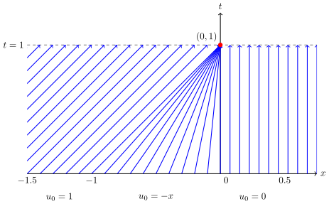
Note that we are forced into this blowup – there is nothing we can do to avoid it. As soon as our initial data has a decreasing section, the dynamics of the equation itself force our hand. This is despite the best regularity assumptions you could ask for; both the space and time components of our spacetime divergence \(u_t+(u^2/2)_x\) are simple polynomials, yet generic solutions blow up in finite time. The reason for this blow-up is that the wave travelling from \(-1\) is faster than the later waves, and thus eventually catches up to them.
The blow-up phenomenon can be made to appear familiar with a little bit of calculus. Differentiating the Burgers equation, and letting \(v=\partial_xu\), we get
\[\partial_tv+u\,\partial_xv=-v^2,\]since \(\partial_x(u\,\partial_xu)=u\,\partial_x(\partial_xu)+(\partial_xu)^2\); note the similarity to the transport equation, apart from the right-hand side term. This transport equation describes the evolution of \(v\) along the trajectories generated by the transport field \(u\). That is, along the line \((x_0+u_0(x_0)\,t,t)\) in spacetime, consider the function \(v(t;x_0)=v(x_0+u_0(x_0)\,t,t)\), where the notation \((t;x_0)\) indicates that the function is of a single variable, \(t\), but is indexed by space points \(x_0\in\mathbb R\), i.e. each \(x_0\) yields such a function. As defined, \(v(t)\) satisfies the Riccati equation (with flipped sign)
\[v^{\prime}(t)=-v(t)^2,\]which we saw blows up at \(T^*=-v(0)^{-1}\) if \(v(0)<0\); this is precisely the condition that \(u_0^\prime<0\) somewhere. Thus, the blow-up of the derivative is governed by precisely the same mechanism as the Riccati equation we pondered earlier! Is there any way to rescue these equations?
One hope comes from something we ignored before – friction. We can imagine friction damping the motion of moving bodies, and here in the form of viscosity it will have a similar effect on controlling blow-up. We will also see that the slightest bit of friction is sufficient. Of course, this analogy is imperfect, because viscosity is a different kind of friction – it pulls nearby schmuid packets toward similar speeds, and thus fights against the steepening of the wave profile. A simple exercise of the chain rule tells us that the Burgers equation can equivalently be written as a spacetime divergence equation of the form
\[\partial_tu+\partial_x\left(\frac12u^2\right)=0.\]The factor of half ensures that the speed is \(u\) and not \(2u\). Since the wave speed depends on the value of \(u\), schmuid packets travel at different speeds. The fast-travelling packets push against the slower ones and are pushed back in turn. Variation in the ‘flux’ term, here \(\tfrac12u^2\), governs the rate of change of \(u\) in time. To modify this flux with viscous friction, we add \(-\nu\,\partial_xu\) to the flux, which yields the modified conservation law
\[\partial_tu+\partial_x\left(\frac12u^2-\nu\partial_xu\right)=0\]Thus, we obtain the viscous Burgers equation
\[\partial_tu+\partial_x\left(\frac12u^2\right)=\nu\,\partial_{xx}u.\]Let’s see what viscosity can buy us with a fast-moving schmuid packet \(u=u_L\) on the left of \(x=0\) and a slow packet \(u=u_R\) on the right, i.e. \(u_L>u_R\). Without any friction, the fast packet overtakes and causes the wave to break over itself. With only friction, i.e. ignoring the flux term, we get the heat equation in one dimension, which governs the evolution of a temperature distribution. The characteristic feature of heat is that it attempts to smoothen out sharp gradients; in particular solutions to the Cauchy problem for the heat equation are instantaneously made smooth, even if the initial data has discontinuities.
Thus we see two tendencies battling each other out; heat wants to spread the schmuid around, while the convection, or flux term, pushes fast packets into slow ones. It turns out that the effect of the viscous term dominates, and solutions remain smooth. However, the resolution is a truce, and not a total conquest. Heat is not able to flatten out the profile completely, and we obtain a travelling ‘viscous shock wave’ – a profile \(u(x,t)=U(\xi)\) with \(\xi=x-at\) that slides rigidly at some speed \(a\), where \(U\) goes from \(u_L\) far to the left \((-\infty)\) to \(u_R\) far to the right \((+\infty)\). Substituting this into the equation and integrating once yields
\[\nu\,U' = \tfrac12\,(U - u_L)(U - u_R),\]and forces the speed to be the average, \(a= (u_L + u_R)/2\). The transition from \(u_L\) to \(u_R\) happens over a width of roughly \(\nu\) divided by the size of the jump, \(u_L-u_R\). Thus, as the parameter \(\nu\to0\), the viscous travelling wave steepens into a discontinuity as the characteristics picture would suggest.
In one spatial dimension, friction is strong enough to establish the truce with nonlinearity on favourable terms. However, the maximum principle in this case, i.e. the guarantee that \(u\) at future times will never exceed fixed upper and lower limits, plays a key role in ensuring the success of this mechanism. In other settings, bets are off. Viscosity alone may not suffice to save the classical notion of solution. In the Navier-Stokes equations, for instance, the fluid velocity may violate the maximum principle, indeed the blow-up of the velocity itself is a necessary condition for blow-up of the solution. In three dimensions, the controlled quantity, energy, is too weak relative to the supercritical nonlinearity.
Given some ‘divergence free’ initial velocity field \(u_0:\mathbb{R}^d\to\mathbb{R}^d\) and space-time force \(f:\mathbb{R}^d\times\mathbb{R}_{+}\to\mathbb{R}^d\), the Cauchy problem for the incompressible fluid asks to determine its evolution according to the PDE, while satisfying the divergence constraint. Since these equations are nonlinear, blow-up is a nontrivial possibility. The forcing function \(f\) is merely a given function of space and time; even if we restrict ourselves to the case where \(f=0\), and the fluid is pushed around merely by its own internal momentum, the difficulty of analysing the PDE comes primarily from its non-linearity. Note that given a solution \(u\), scaling it by a factor of \(\lambda\in\mathbb{R}\) does not yield another solution, since the second term scales quadratically. Thus, behaviour of the equation should be expected to be more like the nonlinear (viscous) Burgers equation rather than the linear transport equation. Linearity is a very ‘nice’ property for analysts; indeed, the classical notion of a derivative itself is useful precisely because it ‘linearises’ functions around a point.
This is the curse and promise of nonlinearity. As Reuben Hersh writes in Peter Lax, Mathematician: An Illustrated Memoir:
Nonlinearity in mathematical analysis is a complex, fascinating issue that should interest any philosophically minded person. It is comparable to the issue of self-reference and infinite regress in computing and logic and to the issues of positive and negative feedback in engineering. It corresponds to “reflexivity” in George Soros’ writings on finance and economics. The general phenomenon that arises in so many different fields can be described in the following way: something we want to know depends on something else, which depends on the very thing we want to know.
Thus, the existence of solutions itself is a highly non-trivial matter. Technically, we did not know until recently, whether there always exist smooth solutions to the incompressible Navier-Stokes equations (with smooth forcing) defined for arbitrarily large time intervals. If OpenAI’s proof is assumed to be correct, then we know that this is in fact false. There exists a space-time force \(f\) such that the solution \(u\) cannot be defined in the classical sense beyond time \(t=1\), because it ‘blows up’ as the velocity becomes infinite.
At a loose enough level of abstraction, the wave steepening of Burgers equation is similar to that of the incompressible Euler equations; the results announced by OpenAI also include a similar blow-up result for the incompressible Euler equation without any forcing term. However, it is important to not overstate the analogy. For instance, blow-up is not prevented for the Navier-Stokes equations, i.e. ‘viscous Euler’. The precise mechanism of blow-up (vortex stretching) is also quite different. Importantly, it cannot occur in two spatial dimensions; smooth initial data is known to yield global classical solutions to the associated Cauchy problem in this setting.
To paraphrase what Tolstoy said about families, all linear PDEs are alike, and all nonlinear PDEs are nonlinear in their own way. There still are, however, some family resemblances. The slew of blow-up results for equations related to incompressible fluids, such as porous media, Boussinesq, Euler, etc. as established by Alpöge and Buckmaster, building on Córdoba–Martínez-Zoroa, is a testament to this fuzzy notion.
I mentioned above that solutions cannot be defined “in the classical sense” beyond the blow-up time. However, if we sufficiently relax our criteria on what counts as a solution, in particular allowing for rough or even discontinuous solutions to our differential equations, we can obtain a generalised notion of ‘solution’, also known as ‘weak’ solutions. For the Navier-Stokes equations, these are called Leray-Hopf solutions, and have been known to exist globally since 1934. For hyperbolic conservation laws, this leads to the notion of shock solutions, which are my personal specialty. Solutions of the viscous Burgers equation converge to a discontinuous ‘shock’ profile as the viscosity is reduced to zero. This method of ‘vanishing viscosity’ was used in much greater generality by S.N. Kružkov to prove the well-posedness of the Cauchy problem for scalar conservation laws in multiple space dimensions. In a future post, we will go over the notion of weak solutions in the context of the Burgers equation.
P.S. while I was in the process of polishing my post, Diego Córdoba and Luis Martínez-Zoroa published a brilliant guest post explaining blow-up for incompressible equations in greater technical depth. Highly recommended for the rigorously inclined reader.